library(dplyr)
library(tidyr)
library(ggplot2)
library(ggtext)
library(ggbranding)
library(ggrepel)
library(patchwork)
library(showtext)
library(AddFonts)
library(cowplot)
library(magick)
library(readr)
library(stringr)
library(scales)

urban <- read_csv("https://raw.githubusercontent.com/rfordatascience/tidytuesday/main/data/2026/2026-09-22/urban.csv")Average share of green areas across cities
TidyTuesday 2026-09-22
r
ggplot2
tidyverse
data-viz
Overview
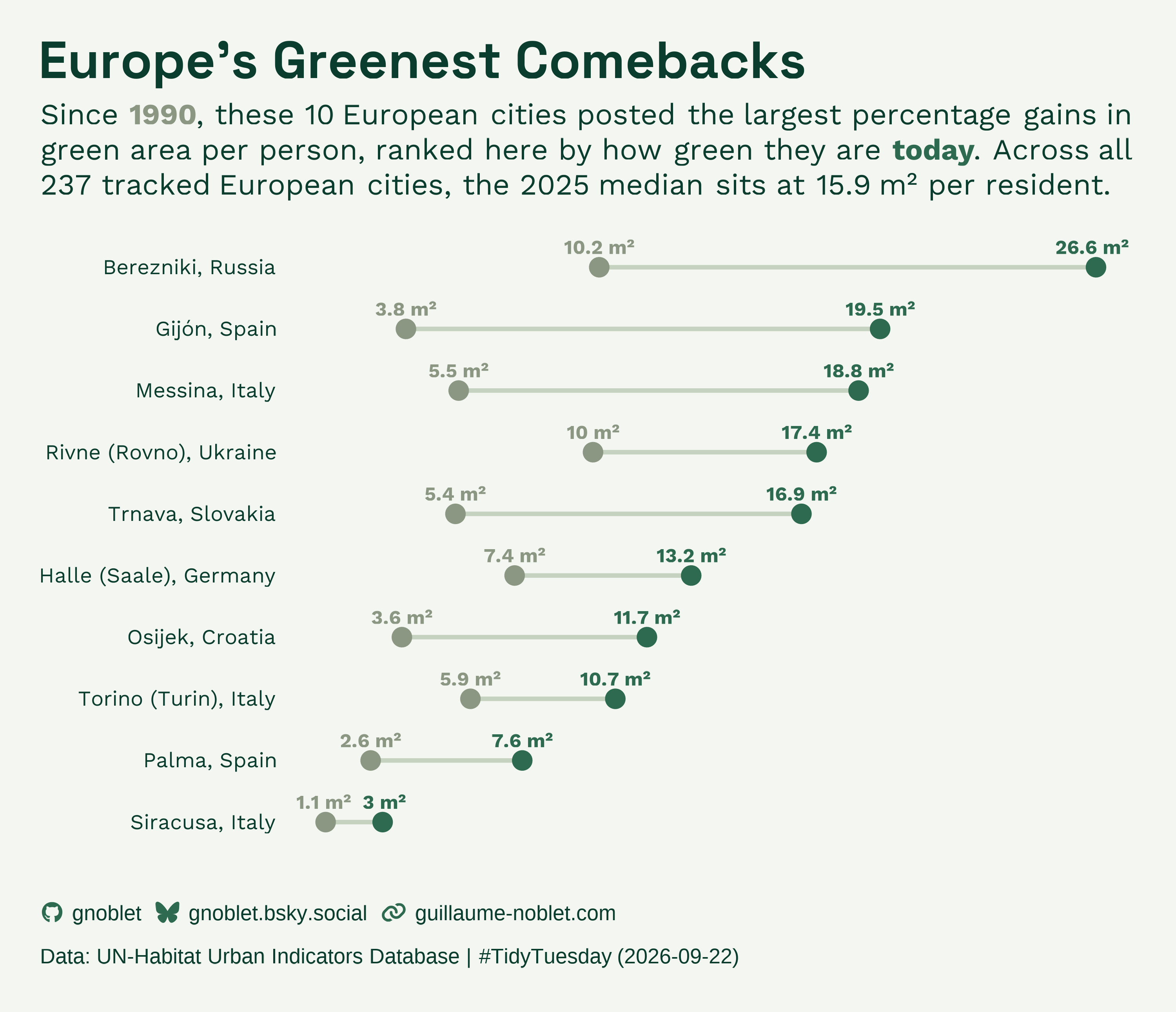
This week’s data comes from the UN-Habitat Urban Indicators Database, which tracks green area per capita for 1,106 cities across 164 countries, surveyed every ten years from 1990 to 2025 (SDG indicator 11.7.1). Europe’s 237 tracked cities all have data in both years, with a 2025 median of about 15.9 m² of green space per resident — a figure that hides huge variation underneath it. Below are the ten European cities whose green area per capita grew the most since 1990, ranked by how green they actually are today.
Tip
Please cite, it’s nice! — Guillaume Noblet (2026). Tidy Tuesday Gallery. https://gnoblet.codeberg.page/TidyTuesday
Visualization
Libraries and Data
european_subregions <- c(
  "Western Europe",
  "Eastern Europe",
  "Northern Europe",
  "Southern Europe"
)

european_cities <- urban |>
  filter(sdgSubRegion %in% european_subregions) |>
  mutate(
    countryOrTerritoryName = if_else(
      countryOrTerritoryName == "Russian Federation", "Russia", countryOrTerritoryName
    )
  )

europe_1990 <- european_cities |>
  filter(year == 1990) |>
  select(cityName, countryOrTerritoryName, sdgSubRegion, greenAreaPerCapitaM2) |>
  rename(greenArea_1990 = greenAreaPerCapitaM2)

europe_2025 <- european_cities |>
  filter(year == 2025) |>
  select(cityName, countryOrTerritoryName, sdgSubRegion, greenAreaPerCapitaM2) |>
  rename(greenArea_2025 = greenAreaPerCapitaM2)

europe_change <- europe_1990 |>
  inner_join(europe_2025, by = c("cityName", "countryOrTerritoryName", "sdgSubRegion")) |>
  # Drop 0 anomalies
  filter(greenArea_1990 > 0, greenArea_2025 > 0) |>
  mutate(percentChange = (greenArea_2025 - greenArea_1990) / greenArea_1990 * 100)

# Top 10 cities by % gain since 1990
# ordered on the chart by how green they are today (greenArea_2025)
top_gain_europe <- europe_change |>
  arrange(desc(percentChange)) |>
  head(10) |>
  mutate(
    cityLabel = paste(cityName, countryOrTerritoryName, sep = ", "),
    cityLabel = forcats::fct_reorder(cityLabel, greenArea_2025)
  )

# Long format so start/end points and labels can be colored and repelled
gain_long <- top_gain_europe |>
  select(cityLabel, greenArea_1990, greenArea_2025) |>
  pivot_longer(
    cols = c(greenArea_1990, greenArea_2025),
    names_to = "period",
    values_to = "greenArea"
  ) |>
  mutate(period = if_else(period == "greenArea_1990", "1990", "2025"))

# Real numbers used in the subtitle/caption below
n_cities_global    <- n_distinct(urban$cityName)
n_countries_global <- n_distinct(urban$countryOrTerritoryName)
n_euro_cities       <- n_distinct(european_cities$cityName)
median_2025_euro    <- median(europe_2025$greenArea_2025, na.rm = TRUE)
# Fonts
title_font <- 'Space Grotesk'
subtitle_font <- 'Work Sans'
main_font <- 'Work Sans'
branding_font <- 'Work Sans'
# Colors
main_color <- '#0B3D2E'
bg_color <- '#F4F7F1'
color_1990 <- '#8b9783'
color_2025 <- '#2D6A4F'
segment_color <- '#c6d2c0'
branding_text_color <- main_color
branding_icon_color <- color_2025
branding_additional_text_color <- main_color
period_colors <- c('1990' = color_1990, '2025' = color_2025)
# Fonts
add_font(main_font)
add_font(title_font)
add_font(branding_font)
showtext_auto()
showtext_opts(dpi = 300)
# Branding
branding <- branding(
github = 'gnoblet',
bluesky = 'gnoblet.bsky.social',
website = 'guillaume-noblet.com',
text_size = '13pt',
icon_size = '13pt',
text_color = branding_text_color,
icon_color = branding_icon_color,
line_spacing = 2L,
text_position = 'after',
additional_text = "Data: UN-Habitat Urban Indicators Database | #TidyTuesday (2026-09-22)",
additional_text_size = '13pt',
additional_text_color = branding_additional_text_color,
text_family = branding_font
)
# Titles
title <- "Europe's Greenest Comebacks"
subtitle <- str_glue(
"Since <span style='color:{color_1990};'>**1990**</span>, these {nrow(top_gain_europe)} ",
'European cities posted the largest percentage gains in green area per person, ranked here ',
"by how green they are <span style='color:{color_2025};'>**today**</span>. Across all ",
'{scales::comma(n_euro_cities)} tracked European cities, the 2025 median sits at ',
'{round(median_2025_euro, 1)} m² per resident.'
)
# Dumbbell plot: green area per capita, 1990 vs. 2025
p_plot <- ggplot(top_gain_europe, aes(y = cityLabel)) +
geom_segment(
aes(x = greenArea_1990, xend = greenArea_2025, yend = cityLabel),
linewidth = 1.3, color = segment_color
) +
geom_point(
data = gain_long,
aes(x = greenArea, color = period),
size = 5
) +
geom_text_repel(
data = gain_long,
aes(x = greenArea, label = paste0(round(greenArea, 1), ' m²'), color = period),
family = main_font, size = 4.2, fontface = 'bold',
direction = 'x', segment.color = NA, show.legend = FALSE,
nudge_y = 0.32, seed = 42
) +
scale_color_manual(values = period_colors, name = NULL) +
labs(title = title, subtitle = subtitle, x = NULL, y = NULL) +
theme_minimal_grid(font_size = 15, line_size = 0, font_family = main_font) +
theme(
text = element_text(color = main_color),
axis.text = element_text(color = main_color),
axis.text.x = element_blank(),
plot.title.position = 'plot',
plot.title = ggtext::element_textbox_simple(
family = title_font, face = 'bold', color = main_color,
size = 32, margin = margin(b = 10)
),
plot.subtitle = ggtext::element_textbox_simple(
family = subtitle_font, color = main_color,
size = 18, lineheight = 1.2, margin = margin(b = 18)
),
legend.position = 'none',
panel.grid.major.y = element_blank(),
panel.grid.minor = element_blank(),
plot.background = element_rect(fill = bg_color, color = NA),
panel.background = element_rect(fill = bg_color, color = NA),
plot.margin = margin(20, 20, 8, 20)
)
p_footer <- ggplot() +
geom_textbox(
aes(label = branding),
x = 0, y = 0.45, hjust = 0, vjust = 0.5, fill = NA, box.color = NA,
box.padding = unit(c(0, 0, 0, 0), 'pt'), width = unit(0.65, 'npc')
) +
coord_cartesian(xlim = c(0, 1), ylim = c(0, 1), expand = FALSE) +
theme_void() +
theme(
plot.background = element_rect(fill = bg_color, color = NA),
plot.margin = margin(4, 20, 16, 20)
)
p <- (p_plot / wrap_elements(full = p_footer)) +
plot_layout(heights = c(1, 0.17)) &
theme(plot.background = element_rect(fill = bg_color, color = NA))ggsave(
'week_38.png',
plot = p,
width = 10,
height = 8.6,
dpi = 300,
bg = bg_color
)
image <- image_read('week_38.png')
image <- image_scale(image, geometry_size_pixels(width = 500, preserve_aspect = TRUE))
image_write(image, 'week_38_thumb.png', format = 'png')