library(dplyr)
library(tidyr)
library(readr)
library(stringr)
library(ggplot2)
library(ggtext)
library(ggrepel)
library(ggbranding)
library(showtext)
library(AddFonts)
library(patchwork)
library(sf)
library(rnaturalearth)
library(magick)

dat <- read_csv("https://raw.githubusercontent.com/rfordatascience/tidytuesday/main/data/2026/2026-09-01/world_castles.csv")World Castles, Fortresses and Palaces
TidyTuesday 2026-09-01
r
ggplot2
tidyverse
data-viz
Overview
This week we’re exploring the Castlemap dataset of 5,793 castles, fortresses, palaces and ruins in 138 countries. The data comes from Wikidata, and every landmark has verified coordinates, a Wikipedia article and a photo on Wikimedia Commons. Each also has a fame rank, based on how many languages have an article on it and how often that article is read. The Great Wall of China is first.
Tip
Please cite, it’s nice! — Guillaume Noblet (2026). Tidy Tuesday Gallery. https://gnoblet.codeberg.page/TidyTuesday
Visualization
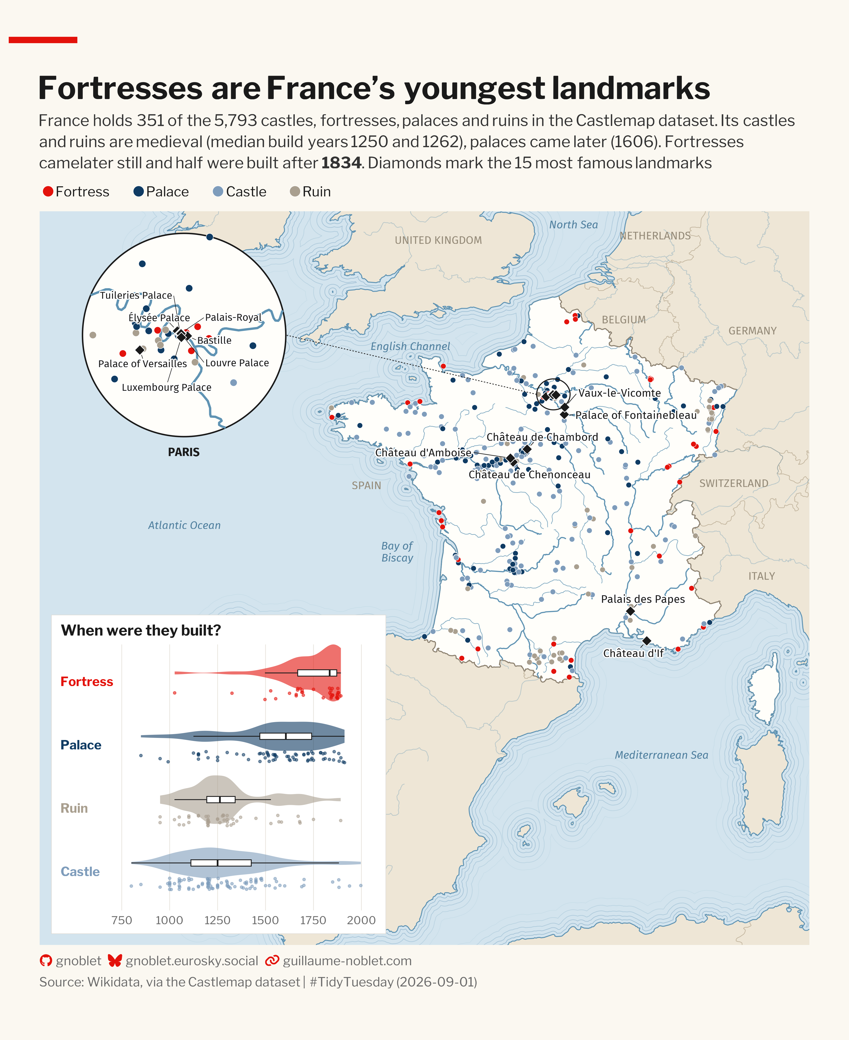
Libraries and Data
# Map bbox: space in atlantic ocean for Paris zoom in and violin plot
xmin_fr <- -14
xmax_fr <- 10.5
ymin_fr <- 36.4
ymax_fr <- 53

# Keep France only
castles_fr <- dat |> filter(country == "France")

# Planar geometry is fine at this scale
sf_use_s2(FALSE)

# Land is cropped a degree wider than the map, so the cut edges fall outside the frame
crop_wide <- function(x) {
  st_crop(x, xmin = xmin_fr - 1, xmax = xmax_fr + 1, ymin = ymin_fr - 1, ymax = ymax_fr + 1)
}

world_crop  <- crop_wide(ne_download(scale = 10, type = "countries", category = "cultural", returnclass = "sf", load = TRUE))
france_poly <- world_crop |> filter(ADMIN == "France")
land        <- st_union(world_crop)
coastline   <- st_boundary(land)

# Water lines: rings rippling off all coasts, fading out as they enter the sea.
water_lines <- purrr::map(c(8, 17, 28, 42, 60), function(km) {
  ring <- st_transform(land, 3035) |> st_buffer(km * 1000) |> st_boundary() |> st_transform(4326)
  st_sf(km = km, geometry = ring)
}) |>
  purrr::list_rbind()

# Major rivers plus Natural Earth's supplementary European rivers
read_rivers <- function(type, size) {
  r <- ne_download(scale = 10, type = type, category = "physical", returnclass = "sf", load = TRUE)
  st_sf(size = size, geometry = st_geometry(st_make_valid(r)))
}
rivers_fr <- rbind(
  read_rivers("rivers_europe", "minor"),
  read_rivers("rivers_lake_centerlines", "major")
) |>
  crop_wide()

# France river details
rivers_france <- st_intersection(rivers_fr, st_geometry(france_poly))

# Most famous landmarks
famous <- castles_fr |>
  filter(!is.na(fame_rank)) |>
  arrange(fame_rank) |>
  slice_head(n = 15)

# Paris loupe. Paris is far too dense to read at national scale
paris_lon   <- 2.3522
paris_lat   <- 48.8566
paris_r_deg <- 0.35
paris_rx    <- paris_r_deg / cos(paris_lat * pi / 180)

lon_scale <- cos(mean(c(ymin_fr, ymax_fr)) * pi / 180)
loupe_x   <- -9.4
loupe_y   <- 50.2
loupe_r   <- 2.3
mag       <- loupe_r / paris_r_deg

to_loupe_x <- function(lon) loupe_x + mag * (lon - paris_lon) * cos(paris_lat * pi / 180) / lon_scale
to_loupe_y <- function(lat) loupe_y + mag * (lat - paris_lat)

in_paris <- function(lon, lat) ((lon - paris_lon) / paris_rx)^2 + ((lat - paris_lat) / paris_r_deg)^2 <= 1

circle <- function(cx, cy, rx, ry, n = 240) {
  t <- seq(0, 2 * pi, length.out = n)
  tibble(x = cx + rx * cos(t), y = cy + ry * sin(t))
}

paris_ring <- circle(paris_lon, paris_lat, paris_rx, paris_r_deg)
loupe_disc <- circle(loupe_x, loupe_y, loupe_r / lon_scale, loupe_r)

castles_paris <- castles_fr |>
  filter(in_paris(lon, lat)) |>
  mutate(x = to_loupe_x(lon), y = to_loupe_y(lat))

paris_labels <- castles_paris |>
  filter(!is.na(fame_rank)) |>
  arrange(fame_rank) |>
  slice_head(n = 7)

# The Seine through Paris
paris_window <- st_sfc(st_polygon(list(as.matrix(paris_ring))), crs = 4326)
seine <- st_intersection(st_geometry(rivers_fr |> filter(size == "major")), paris_window)
seine_loupe <- (seine - c(paris_lon, paris_lat)) *
  diag(c(mag * cos(paris_lat * pi / 180) / lon_scale, mag)) + c(loupe_x, loupe_y)
seine_loupe <- st_set_crs(seine_loupe, 4326)

# Thin leader from the Paris ring to the loupe
loupe_link <- tibble(
  x = paris_lon - paris_rx, y = paris_lat,
  xend = loupe_x + loupe_r / lon_scale, yend = loupe_y
)

famous <- famous |> mutate(paris = in_paris(lon, lat))

# Construction years for the raincloud chart.
# Remove the few very early ruins (before 1000 BCE) to not stretch the axis too much
year_dat <- castles_fr |>
  filter(!is.na(year), year >= -1000) |>
  mutate(category = stats::reorder(category, year, FUN = median))

set.seed(35)
rain_dat <- year_dat |>
  slice_sample(n = 300, by = category) |>
  mutate(x_jitter = as.numeric(category) - 0.18 + stats::runif(n(), -0.09, 0.09))

medians <- year_dat |> summarise(med = round(median(year)), .by = category)
med_of  <- function(cat) medians$med[medians$category == cat]

country_counts <- dat |> count(country, sort = TRUE)
france_rank <- which(country_counts$country == "France")

# Map annotations: neighbours in capitals, seas in italics
country_names <- tribble(
  ~label,            ~lon,  ~lat,
  "UNITED KINGDOM",  -1.3,  52.35,
  "NETHERLANDS",      5.6,  52.45,
  "BELGIUM",          4.6,  50.55,
  "GERMANY",          8.7,  50.3,
  "SWITZERLAND",      8.1,  46.85,
  "ITALY",            9.0,  44.75,
  "SPAIN",           -3.6,  46.8,
  "PORTUGAL",        -8.3,  39.15
)
sea_names <- tribble(
  ~label,              ~lon,  ~lat,
  "Atlantic Ocean",   loupe_x, loupe_y - loupe_r - 2,
  "Bay of\nBiscay",    -2.6,  45.3,
  "English Channel",   -2.2,  49.95,
  "North Sea",          3.0,  52.7,
  "Mediterranean Sea",  5.8,  40.7
)
# Fonts
main_font <- 'Libre Franklin'
map_font <- 'Fira Sans'
add_font(main_font)
add_font(map_font)
showtext_auto()
showtext_opts(dpi = 300)
# Atlas palette:
page <- '#FBF8F1'
ink <- '#1A1A1A'
muted <- '#6B6B6B'
sea <- '#D3E4EE'
water <- '#5F93B3'
neighbour <- '#EEE6D6'
france <- '#FFFEFA'
border <- '#C4B7A0'
red <- '#E3120B'
category_palette <- c(
fortress = red,
palace = '#0F3B63',
castle = '#7E9CBB',
ruin = '#A99F8F'
)
category_order <- c('fortress', 'palace', 'castle', 'ruin')
title <- "Fortresses are France's youngest landmarks"
subtitle <- str_glue(
"France holds {nrow(castles_fr)} of the 5,793 castles, fortresses, palaces and ruins in the Castlemap ",
"dataset. Its castles and ruins are medieval (median build years ",
"{med_of('castle')} and {med_of('ruin')}), palaces came later ({med_of('palace')}). Fortresses came",
"later still and half were built after **{med_of('fortress')}**. Diamonds mark the 15 most famous landmarks"
)
caption <- branding(
github = 'gnoblet', bluesky = 'gnoblet.eurosky.social', website = 'guillaume-noblet.com',
additional_text = paste(
'Source: Wikidata, via the Castlemap dataset | #TidyTuesday (2026-09-01)',
sep = '<br>'
),
text_position = 'after', line_spacing = 2L,
text_color = muted, icon_color = red, additional_text_color = muted,
text_size = '13pt', icon_size = '13pt', additional_text_size = '13pt'
)
p_map <- ggplot() +
# Sea
geom_sf(data = water_lines, aes(alpha = km), colour = water, linewidth = 0.3) +
scale_alpha(range = c(0.45, 0.08), guide = 'none') +
# Land
geom_sf(data = world_crop, fill = neighbour, colour = border, linewidth = 0.3) +
geom_sf(data = france_poly, fill = france, colour = '#8C8170', linewidth = 0.5) +
# Rivers
geom_sf(data = rivers_fr |> filter(size == 'major'), colour = water, alpha = 0.35, linewidth = 0.35) +
geom_sf(data = rivers_france |> filter(size == 'minor'), colour = water, alpha = 0.8, linewidth = 0.3) +
geom_sf(data = rivers_france |> filter(size == 'major'), colour = water, linewidth = 0.55) +
# Coastline
geom_sf(data = coastline, colour = water, linewidth = 0.45) +
# Country labels
geom_text(
data = country_names, aes(lon, lat, label = label),
family = map_font, colour = '#948A78', size = 4
) +
# Sea labels
geom_text(
data = sea_names, aes(lon, lat, label = label),
family = map_font, fontface = 'italic', colour = '#4F7F9E', size = 4, lineheight = 0.9
) +
# Castles
geom_point(
data = castles_fr |> mutate(category = factor(category, category_order)),
aes(lon, lat, fill = category),
shape = 21, size = 2.4, colour = 'white', stroke = 0.3
) +
# Famous castles
geom_point(
data = famous, aes(lon, lat),
shape = 23, size = 3.6, fill = ink, colour = 'white', stroke = 0.5
) +
# Keep the national labels off the ring
geom_text_repel(
data = bind_rows(
famous |> filter(!paris) |> select(lon, lat, name),
paris_ring |> slice(seq(1, n(), by = 12)) |> mutate(lon = x, lat = y, name = '', .keep = 'none')
),
aes(lon, lat, label = name),
family = map_font, size = 4, colour = ink,
box.padding = 0.5, point.padding = 0.3, segment.colour = ink, segment.size = 0.3,
min.segment.length = 0, max.overlaps = Inf, seed = 35,
bg.color = 'white', bg.r = 0.15
) +
# Paris ring, leader and loupe
geom_path(data = paris_ring, aes(x, y), colour = ink, linewidth = 0.5) +
geom_segment(
data = loupe_link, aes(x = x, y = y, xend = xend, yend = yend),
colour = ink, linewidth = 0.35, linetype = '22'
) +
geom_polygon(data = loupe_disc, aes(x, y), fill = france, colour = ink, linewidth = 0.7) +
geom_sf(data = seine_loupe, colour = water, linewidth = 1.1) +
geom_point(
data = castles_paris |> mutate(category = factor(category, category_order)),
aes(x, y, fill = category),
shape = 21, size = 3.2, colour = 'white', stroke = 0.3
) +
geom_point(
data = paris_labels, aes(x, y),
shape = 23, size = 3.6, fill = ink, colour = 'white', stroke = 0.5
) +
geom_text_repel(
data = paris_labels, aes(x, y, label = name),
family = map_font, size = 3.6, colour = ink,
box.padding = 0.55, point.padding = 0.3, force = 3, segment.colour = ink, segment.size = 0.25,
min.segment.length = 0, max.overlaps = Inf, seed = 35,
bg.color = 'white', bg.r = 0.15,
xlim = loupe_x + c(-1, 1) * 0.92 * loupe_r / lon_scale,
ylim = loupe_y + c(-1, 1) * 0.92 * loupe_r
) +
annotate(
'text', x = loupe_x, y = loupe_y - loupe_r - 0.35, label = 'PARIS',
family = map_font, fontface = 'bold', size = 4.2, colour = ink
) +
# Legend
scale_fill_manual(
values = category_palette, breaks = category_order,
labels = str_to_title(category_order), name = NULL
) +
guides(fill = guide_legend(nrow = 1, override.aes = list(size = 5))) +
# Labels
labs(title = title, subtitle = subtitle, caption = caption) +
coord_sf(xlim = c(xmin_fr, xmax_fr), ylim = c(ymin_fr, ymax_fr), expand = FALSE) +
# Theme
theme_void(base_family = main_font) +
theme(
plot.background = element_rect(fill = page, colour = NA),
panel.background = element_rect(fill = sea, colour = NA),
plot.margin = margin(40, 35, 15, 35),
plot.title.position = 'plot',
plot.caption.position = 'plot',
plot.title = element_textbox_simple(
family = main_font, face = 'bold', size = 32, colour = ink,
lineheight = 1.1, margin = margin(b = 10)
),
plot.subtitle = element_textbox_simple(
family = main_font, size = 16, colour = '#333333', lineheight = 1.35, margin = margin(b = 12)
),
plot.caption = element_textbox_simple(
family = main_font, colour = muted, halign = 0, margin = margin(t = 10)
),
legend.position = 'top',
legend.justification = 'left',
legend.text = element_text(family = main_font, size = 14, colour = ink, margin = margin(r = 14)),
legend.key = element_rect(fill = NA, colour = NA),
legend.margin = margin(b = 6)
)
# Raincloud chart: half-violins with a narrow boxplot, and the raw years as rain underneath.
cat_label <- function(x) sprintf("<span style='color:%s'>**%s**</span>", category_palette[x], str_to_title(x))
p_inset <- ggplot(year_dat, aes(x = category, y = year)) +
geom_violin(
aes(fill = category), trim = TRUE, alpha = 0.6, colour = NA,
position = position_nudge(x = 0.15), width = 0.9
) +
geom_boxplot(
width = 0.1, outlier.shape = NA, linewidth = 0.4, fill = 'white', colour = ink,
position = position_nudge(x = 0.15)
) +
geom_point(
data = rain_dat, aes(x = x_jitter, y = year, colour = category),
inherit.aes = FALSE, size = 0.9, alpha = 0.55
) +
scale_fill_manual(values = category_palette, guide = 'none') +
scale_colour_manual(values = category_palette, guide = 'none') +
scale_x_discrete(labels = cat_label) +
coord_flip() +
labs(
title = 'When were they built?',
x = NULL, y = NULL
) +
theme_minimal(base_size = 13, base_family = main_font) +
theme(
plot.background = element_rect(fill = 'white', colour = '#D8D4CC', linewidth = 0.4),
panel.grid.major.y = element_blank(),
panel.grid.minor = element_blank(),
panel.grid.major.x = element_line(colour = '#E6E2DA', linewidth = 0.3),
# coord_flip draws the category axis with axis.text.y.left, which is
# plain text in the base theme, so the markdown element goes there
axis.text.y.left = element_markdown(size = 13, hjust = 0),
axis.text.x = element_text(colour = muted, size = 11),
plot.title = element_text(face = 'bold', size = 15, colour = ink),
plot.title.position = 'plot',
plot.margin = margin(10, 14, 8, 10)
)
# Red tab at the top-left
red_tab <- ggplot() +
annotate('rect', xmin = 0, xmax = 1, ymin = 0, ymax = 1, fill = red) +
theme_void()
# Hop final insetting
p <- p_map +
inset_element(p_inset, left = 0.015, right = 0.45, bottom = 0.015, top = 0.45, align_to = 'panel') +
inset_element(red_tab, left = 0, right = 0.09, bottom = 0.993, top = 1, align_to = 'full') +
plot_annotation(theme = theme(plot.background = element_rect(fill = page, colour = NA)))ggsave(
'week_35.png',
plot = p,
width = 12,
height = 14.7,
dpi = 300,
bg = page
)
image <- image_read('week_35.png')
image <- image_scale(image, geometry_size_pixels(width = 500, preserve_aspect = TRUE))
image_write(image, 'week_35_thumb.png', format = 'png')