Day 07: Outliers

library(HistData)
library(tidyverse)
library(outliers)     # For Grubbs' test
library(DMwR2)        # For LOF
library(solitude)     # For Isolation Forest
library(EnvStats)     # For Rosner's test
library(ggplot2)
library(showtext)
library(sysfonts)
library(ggtext)
library(Cairo)

data(Pollen)

# Prepare data
dat <- Pollen

# Outlier flagging
outlier_flags <- dat |>
  mutate(
    # 1. Grubbs' Test
    Grubbs = {
      test <- grubbs.test(density)
      ifelse(density == ifelse(grepl("highest", test$alternative),
                            max(density), min(density)),
             test$p.value < 0.05, FALSE)
    },

    # 2. IQR (1.5x)
    IQR = density %in% boxplot.stats(density)$out,

    # 3. Z-score (>3)
    Zscore = abs(scale(density)) > 3,

    # 4. Hampel Filter (3 MAD)
    Hampel = abs(density - median(density)) > 3 * mad(density),

    # 5. Modified Z-score (>3.5)
    ModZscore = (0.6745 * (density - median(density))) / mad(density) > 3.5,

    # 6. Isolation Forest
    ISO_Forest = {
        iso <- isolationForest$new(sample_size = 50)  # Reduced from default 256
        iso$fit(data.frame(density = density))
        iso$predict(data.frame(density = density))$anomaly_score > 0.65
    },

    # 7. Local Outlier Factor (LOF)
    LOF = lofactor(density, k = 5) > 1.5,

    # 8. Tukey's Fences (3x IQR)
    Tukey = {
      q <- quantile(density)
      iqr <- IQR(density)
      density < (q[1] - 3*iqr) | density > (q[3] + 3*iqr)
    },

    # 9. Rosner's Test (10 potential outliers)
    Rosner = density %in% (rosnerTest(density, k = 10)$all.stats$Value),

    # 10. 4 Sigma Rule
    Four_Sigma = abs(density - mean(density)) > 4 * sd(density)
  )

# Count # of outliers to order counts by methods
outlier_counts <- outlier_flags |>
  pivot_longer(cols = Grubbs:Four_Sigma,
               names_to = "Method", values_to = "Outlier") |>
  group_by(Method) |>
  summarize(Count = sum(Outlier)) |>
  arrange(desc(Count))
outlier_flags <- outlier_flags |>
  pivot_longer(
    cols = Grubbs:Four_Sigma,
    names_to = "Method", values_to = "Outlier") |>
  mutate(Method = factor(
    Method,
    levels = outlier_counts$Method,
    ordered = TRUE))

# Plot
outlier_flags |>
  ggplot(aes(x = ridge, y = density)) +
  # Plot non-outliers first with transparency
  geom_point(data = ~subset(., !.$Outlier), aes(color = Outlier), size = 1.5, alpha = 0.6) +
  # Overlay outliers with transparency and distinct color
  geom_point(data = ~subset(., .$Outlier), aes(color = Outlier), size = 1.5, alpha = 0.8) +
  geom_smooth(data = ~subset(., !.$Outlier), method = "loess", color = "#415161", lwd = 0.4, level = 0.99) +
  facet_wrap(~ Method, ncol = 2, scales = "free_y") +
  scale_color_manual(values = c("#D3D3D3", "#3498db")) +
  labs(
    title = "<span style='font-size:22pt; color:#415161; font-weight:700'>DETECTING OUTLIERS OF POLLEN DENSITY</span><br>
            <span style='font-size:18pt; color:#3498db'>One-Dimensional Methods Ranked by the Most Outliers Found First</span>",
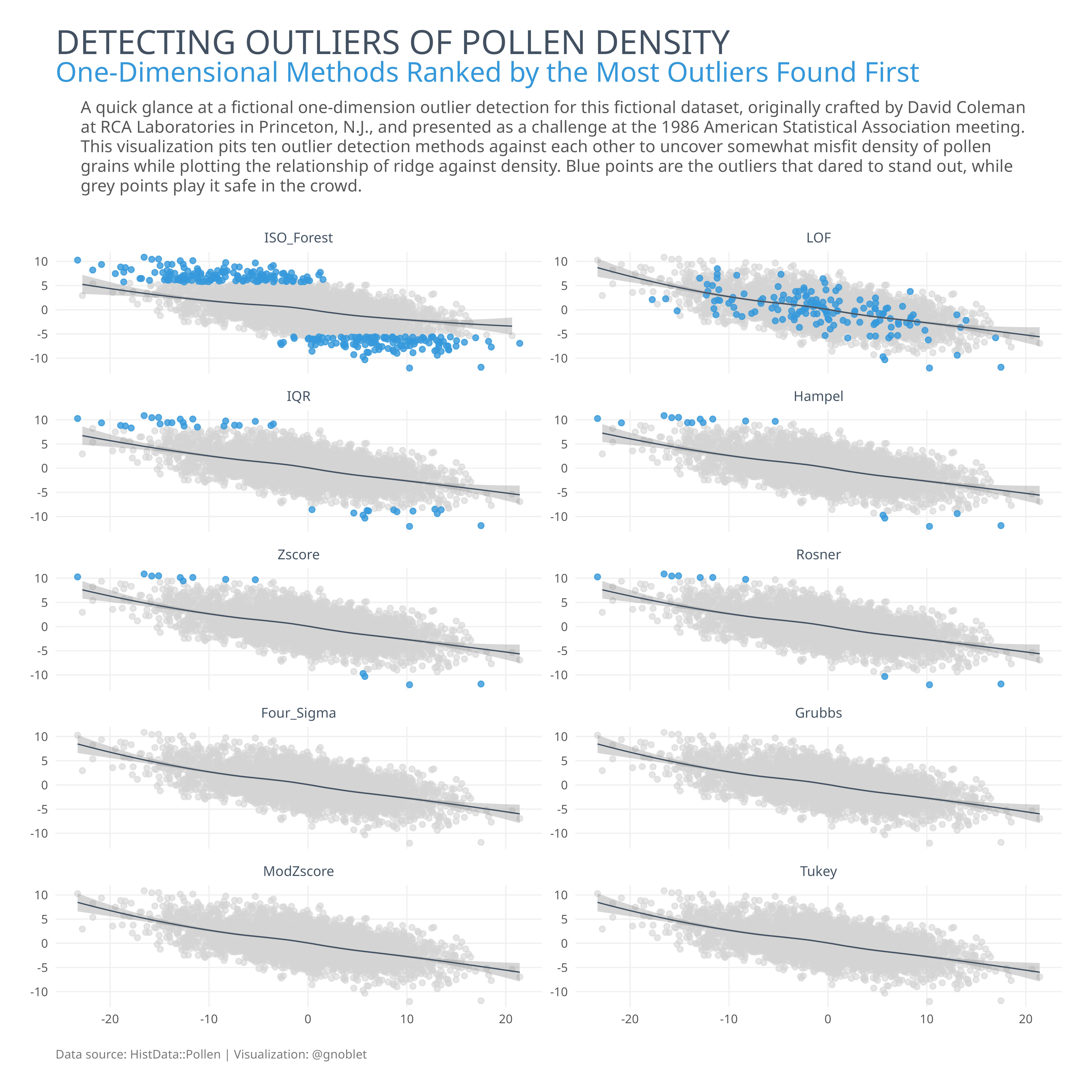
    subtitle = "<span style='color:#555555; font-size:11pt'>A quick glance at a fictional one-dimension outlier detection for this fictional dataset, originally crafted by David Coleman at RCA Laboratories in Princeton, N.J., and presented as a challenge at the 1986 American Statistical Association meeting. This visualization pits ten outlier detection methods against each other to uncover somewhat misfit density of pollen grains while plotting the relationship of ridge against density. Blue points are the outliers that dared to stand out, while grey points play it safe in the crowd.</span>",
    caption = "<span style='color:#777777; font-size:8pt'>Data source: HistData::Pollen | Visualization: @gnoblet</span>"
  ) +
  theme_minimal() +
  theme(
    legend.position = "none",
    strip.text = element_text(
      size = 9,
      color = "#415161",
      margin = margin(5,0,5,0)
    ),
    plot.title = element_textbox_simple(
      padding = margin(0, 0, 5, 0),
      lineheight = 1.2,
      halign = 0
    ),
    plot.subtitle = element_textbox_simple(
      size = 10,
      lineheight = 1.3,
      padding = margin(10, 0, 25, 0),
      width = grid::unit(0.95, 'npc'),
      halign = 0
    ),
    plot.caption = element_textbox_simple(
      hjust = 1,
      margin = margin(15,0,0,0),
    ),
    axis.text.x = element_text(
      size = 8,
      color = "#555555"
    ),
    axis.text.y = element_text(
      size = 8,
      color = "#555555"
    ),
    axis.title.x = element_blank(),
    axis.title.y = element_blank(),
    panel.background = element_rect(fill = "white", color = NA),
    panel.grid.major = element_line(color = "#f0f0f0", linewidth = 0.4),
    panel.grid.minor = element_blank(),
    plot.margin = margin(20,20,20,20),
    plot.background = element_rect(fill = "white")
  )

 # save
ggsave(
  "day_07.png",
  dpi = 600,
  width = 10,
  height = 10,
)

Final Plot

Notes

This visualization compares ten different outlier detection methods applied to pollen density data, ranking them by the number of outliers identified.

Data source: HistData::Pollen dataset (originally from David Coleman at RCA Laboratories)

Tools used:

• outliers (for Grubbs’ test)
• DMwR2 (for Local Outlier Factor)
• solitude (for Isolation Forest)
• EnvStats (for Rosner’s test)
• ggplot2 (for visualization)
• ggtext (for rich text annotations)

The visualization uses a small multiples approach with facets for each outlier detection method. Each panel shows the relationship between ridge and density measurements, with detected outliers highlighted in blue and a smoothed trend line fitted to the non-outlier points. This approach allows for visual comparison of how different statistical methods identify anomalies in the same dataset, revealing the variations in sensitivity and specificity across techniques.